Uncertainty in Deep Learning, p.1 (Intro)
Introduction
The ability of deep neural networks to produce useful predictions is now abundantly clear in hundreds of different applications and tasks across dozens of absolutely different domains, which are constantly being improved and developed and continue to reshape our world in many ways. In the rapidly evolving landscape of deep learning, one often-overlooked aspect which is being overshadowed by the unprecedented accuracy and flexibility of neural networks is the model’s confidence in its predictions—its uncertainty. Along with predictions made by the model \(\textbf{y}\) for an input \(\textbf{x}\), it is often crucial to assess how confident the model is in these predictions and then use this information for other downstream applications.
The problem is not just of interest to academia, but often brings significant value to practical applications ranging from medical to self-driving, which we will cover further. One of the most important areas where uncertainty methods could be used is in safety-critical applications, where we must guarantee the accuracy of the predictions made by the network. As an example, consider the 2016 [incident] where an autonomous driving system tragically misidentified the side of a trailer as the bright sky. These are not just failures in object recognition but failures in assessing the model’s own confidence.

Another example involves the numerous regulations and guidelines that apply to medical diagnoses made using neural networks and other forms of artificial intelligence. The specific regulations can vary significantly by country and region, but several key principles are generally observed worldwide. Regulatory bodies often impose requirements related to the performance of medical devices, which can include metrics like false positive rates. These can be achieved by rejecting unconfident and potentially erroneous predictions.
In the context of large language models (LLMs), addressing alignment, hallucinations, and explainable AI (xAI) is critical for enhancing their trustworthiness and effectiveness. Alignment ensures that LLMs operate in accordance with human values and intentions, helping to prevent adverse outcomes. Hallucinations, where models generate incorrect or nonsensical outputs, pose a significant challenge. Recent research highlights their impact on model reliability, particularly in domains where factual accuracy is crucial. Additionally, explainable AI (xAI) seeks to clarify complex model decisions, making them more transparent and understandable to users. This transparency is especially important in sectors like healthcare and finance, where understanding the reasoning behind model decisions is essential for trust, adoption, and ethical application.
As we will explore further, excessive reliance on neural networks without proper management can be a critical misstep, potentially resulting in undesirable or even catastrophic outcomes. Blindly relying on technology without understanding its inner workings and limitations is a risky approach that can lead to unintended consequences. This is one of the reasons why the topic of model uncertainty and interpretability is becoming increasingly relevant and popular, gaining significant attention from major players such as [OpenAI], [xAI], [Google], [DeepMind], and many others.

In this series, we will cover the topic of uncertainty estimation for deep learning, current challenges and approaches to the task, discuss its applications, and modern developments. I aim to delve deeply into many of these topics, so the reader should expect a considerable amount of formulas and technical details (hopefully, this does not scare you away). The major reason for me to write this series is to share my accumulated knowledge of the topic and also demystify some popular misconceptions and misunderstandings. Since the text above should have given you a good answer to the question “why?” care about uncertainty, what follows will address the “how?”. In this part, we will cover the formal definition of the tasks, discuss the forms that uncertainty estimation can take, and touch on the topic of probabilistic modeling and its connection to modern neural networks.
Problem Definition
Understanding and managing uncertainty is a fundamental challenge in machine learning, particularly as models are deployed in real-world scenarios where predictions can significantly impact decision-making. Uncertainty arises from various sources, including the inherent randomness in data, limitations of the models themselves, and unfamiliar inputs encountered during deployment.
Addressing these challenges requires a comprehensive framework that can quantify, interpret, and act upon different forms of uncertainty. In the following sections, we explore key concepts and approaches in uncertainty estimation, setting the foundation for robust and reliable machine learning systems.
Probabilistic Modelling
Probabilistic modeling lies at the core of many widely used machine learning approaches and serves as one of the cornerstone concepts underpinning modern deep learning models, even if its significance is sometimes overlooked.
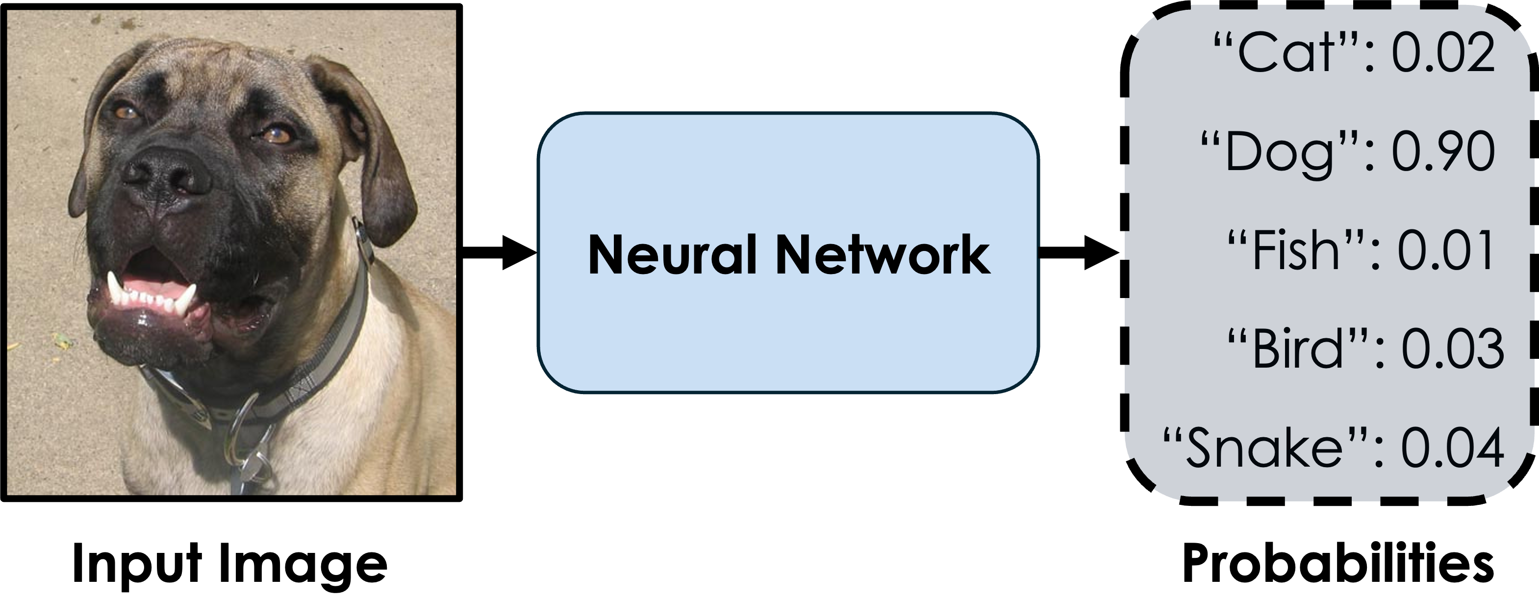
In simple terms, a probabilistic model goes beyond providing single-point estimates for outputs, such as a specific value or label, and instead seeks to represent the entire distribution of possible outcomes [Bis06]. This allows the model to quantify not only the most likely prediction but also the uncertainty or confidence associated with it. For instance, instead of predicting a single temperature value for tomorrow, a probabilistic model might provide a range of likely temperatures along with their respective probabilities. From this perspective, even a simple image classification model can be viewed as a probabilistic model \(P_{\theta}(\textbf{y} \mid \textbf{x})\), parameterized by weights \(\theta\). For a given image x, the model predicts a probability distribution over the possible classes rather than a single deterministic output. This represents a straightforward example of discriminative probabilistic learning.
On the other hand, generative models aim to model the distribution of the data itself, \(P_{\theta}(\textbf{x})\), allowing for the generation of new samples that resemble the original data. A prime example of such models is diffusion models, which gradually transform random noise into realistic images by learning the underlying data distribution. These models belong to the category of generative probabilistic modeling, focusing on capturing the complexities of the data distribution \(P(\textbf{x})\) to facilitate tasks such as image generation, inpainting, molecular design, and other similar applications.
The common feature of both types of probabilistic models mentioned above is their aim to capture the underlying data distribution. This can be done explicitly, as in discriminative models, which focus on modeling conditional probabilities like \(P(\textbf{y} \mid \textbf{x})\), or more implicitly, as in generative models such as GANs [GPM+20] or diffusion models [HJA20], which prioritize capturing \(P(\textbf{x})\) in a manner particularly suited for sampling and data generation.
While uncertainty estimation is closely related to probabilistic modeling, it can be viewed as a specialized subset of probabilistic models that often focus on solving narrower types of problems. In general, when we discuss uncertainty estimation methods, we are typically referring to techniques that operate alongside common discriminative models. In this context, the model produces a prediction \(\textbf{y}\), and the goal is to assess how confident the model is in that prediction. A model’s uncertainty can stem from various sources, such as the inherent complexity of the data distribution or, for example, the lack of sufficient or diverse training data. We explore these types of uncertainties in more detail below.
Uncertainty Types
Uncertainty in machine learning predictions can be categorized into distinct types, each stemming from specific sources within the modeling process. Understanding these uncertainties offers valuable insights into prediction reliability and plays a crucial role in diverse applications.
While more detailed and complex taxonomies exist, most discussions emphasize two primary types of uncertainty: aleatoric (what we know we do not know) and epistemic (what we do not know we do not know) uncertainty. These two categories capture fundamentally different sources of uncertainty, and other forms of uncertainty can often be expressed in terms of these two main types. In the next series, we will formally explore a natural approach to deriving these two types of uncertainties within a Bayesian probabilistic framework.
Aleatoric Uncertainty
Aleatoric uncertainty [HW21] arises from inherent randomness or noise in the data itself. This type of uncertainty is irreducible because it reflects variability that cannot be eliminated even with perfect modeling or infinite data [KG17]. Examples of aleatoric uncertainty include sensor noise in measurements or unpredictable environmental conditions in real-world data collection. Quantifying aleatoric uncertainty is crucial for tasks where noisy data is common, as it helps to gauge the reliability of model predictions.
In formal terms, we can express this as follows: considering the data generation process \(P(\textbf{y}, \textbf{x})\), if for a given x, the conditional distribution \(P(\textbf{y} \mid \textbf{x})\) is flat or uniform—characterized by high entropy in the case of classification or high variance in the case of regression—we refer to this as a situation with high aleatoric uncertainty. This indicates that it is difficult to associate a specific target \(\textbf{y}\) with the given \(\textbf{x}\). Conversely, if \(P(\textbf{y} \mid \textbf{x})\) exhibits low entropy or variance, indicating a strong correspondence between \(\textbf{x}\) and \(\textbf{y}\), we have a case of low aleatoric uncertainty.
Let us consider a real-world example of an image classification task: designing a model to classify images as either “Cat” or “Dog” (with no other possible classes). To achieve this, we collect a dataset containing thousands of images of cats and dogs. Next, we outsource the labeling process to a popular labeling platform, where labelers are presented with each image and asked to provide one of two possible labels: “Cat” or “Dog”. At the end of the labeling procedure, each image is assigned labels by ten independent labelers.
Now, let us consider several specific examples of labeled images, illustrated in Fig. 7-9 For the first two images, the task is relatively straightforward for the labelers. In Fig. 7, the labelers unanimously agree it depicts a “Cat”, while for Fig. 8 image, all labelers confidently label it as a “Dog”. These cases represent examples of low aleatoric uncertainty, as the empirical class distribution for both images has zero entropy, reflecting complete agreement among labelers.


In contrast, the situation depicted in Fig. 9 is more ambiguous. The image contains both a cat and a dog, leading to significant hesitation among the labelers about which class to assign. As a result, five labelers choose “Cat” and the other five choose “Dog”. This results in a class distribution with maximum possible entropy, indicating high aleatoric uncertainty. This example highlights how aleatoric uncertainty arises when the data itself is inherently ambiguous, making it challenging to assign a definitive label.
In this scenario, it becomes evident why aleatoric uncertainty is considered irreducible, even with additional data. For instance, if instead of ten labelers, one hundred labelers were to provide labels for Fig. 9, it is highly likely that approximately fifty would label it as “Cat” and fifty as “Dog”, resulting in the same level of uncertainty. Similarly, increasing the number of training images in the dataset would not make it easier for labelers—or the model—to determine whether the image belongs to the class “Cat” or “Dog”. This demonstrates that aleatoric uncertainty stems from the inherent ambiguity in the data itself and cannot be reduced merely by increasing the amount of data.


Epistemic Uncertainty
Epistemic uncertainty [KD09], on the other hand, stems from a lack of knowledge about the true underlying data distribution or the model parameters. This uncertainty is reducible and decreases as the model encounters more data or is trained with higher-quality data. Epistemic uncertainty is particularly important for identifying out-of-distribution inputs and improving model generalization, as it highlights areas where the model is less confident due to insufficient information [HG17].
In formal terms, epistemic uncertainty arises from a lack of knowledge about the true relationship between \(\textbf{x}\) and \(\textbf{y}\) due to limited or insufficient data. Considering the data generation process, if, for a given \(\textbf{x}\), different learned model parameters \(\theta\) produce significantly variable predictions for, this indicates high epistemic uncertainty. This variability reflects the model’s uncertainty about because it has not encountered enough data to reliably learn the underlying distribution [LPB17]. Conversely, if the model has been trained on sufficient and diverse data, resulting in low variability across different plausible model parameters \(\theta\), the epistemic uncertainty for \(\textbf{x}\) is small.
Let us revisit our example of image classification from the previous subsection. Assuming that we have already trained our model on the available training data, consider the examples depicted in Fig. 11-13. Fig. 11 shows an animal exhibiting visual features that are a combination of both a cat and a dog—traits that were either absent or insufficiently represented in the training dataset. As a result, the model is unable to make a robust and confident prediction. In this case, epistemic uncertainty is high, and the predictive distribution of the model is expected to be flat. A different situation arises in Fig. 12 and 13, which depict a raccoon and a capybara. These animals were entirely absent from the training dataset and are not considered by the trained model as possible classes. Both of these examples represent out-of-distribution (OOD) [KSM+21] cases, a topic we will discuss in detail later. For these examples, epistemic uncertainty is also expected to be high, with the predictive distribution remaining flat due to the model’s lack of knowledge about such inputs.
Unlike aleatoric uncertainty, epistemic uncertainty can be mitigated by gathering additional data or improving the quality of the training dataset, thereby enhancing the model’s understanding of the data distribution. For instance, in the cases illustrated in Fig. 11-13, the issue of high epistemic uncertainty could be addressed by adding more representative data to the training set and extending the set of classes to include a broader range of potential animals that the model can recognize and classify.


Uncertainty Applications
Uncertainty estimation plays a crucial role in real-world applications, where ensuring reliable predictions and informed decision-making is paramount. By quantifying uncertainty, deep learning models can assess confidence levels in their outputs, enabling more robust deployment in high-stakes environments. Applications of uncertainty estimation are broadly categorized into two key areas: safety and exploration.
Uncertainty for Safety
In safety-critical applications, reliable and confident predictions are essential to prevent catastrophic failures. Uncertainty estimation allows models to quantify their confidence and avoid overconfident errors that can lead to disastrous consequences. A prime example is autonomous driving, where perception models must correctly identify and track objects under varying environmental conditions. If a self-driving system encounters an unfamiliar or ambiguous scenario, high uncertainty can trigger fail-safe mechanisms, such as slowing down, handing control back to a human driver, or requesting additional sensor input.
Similarly, in medical diagnosis, uncertainty-aware models improve patient safety by flagging uncertain predictions for expert review. For instance, deep learning models assisting in radiology can provide confidence scores for detected anomalies, ensuring that ambiguous cases receive further human evaluation. This reduces the risk of misdiagnoses and enhances trust in AI-assisted healthcare. In financial systems, uncertainty-aware models mitigate risks by identifying volatile predictions in credit scoring, fraud detection, and stock market forecasting, preventing decisions based on unreliable outputs.
Beyond these, uncertainty estimation plays a role in robotics, aerospace, and industrial automation, where system failures can have severe consequences. By incorporating uncertainty into predictive models, these domains can ensure safer decision-making and reduce the likelihood of costly or life-threatening errors.
Uncertainty for Exploration
In contrast to safety-focused applications, where uncertainty helps prevent errors, in exploration-based applications, uncertainty serves as a valuable tool for decision-making in environments with incomplete information. This is particularly relevant in fields such as active learning, Bayesian optimization, and reinforcement learning.
Active learning leverages uncertainty to guide data collection, reducing annotation costs while improving model performance. Instead of labeling an entire dataset, an active learning system identifies high-uncertainty samples and prioritizes them for human annotation. This strategy accelerates the learning process by focusing on the most informative data points, which is crucial in domains such as medical imaging and scientific research, where labeled data is scarce or expensive to obtain.
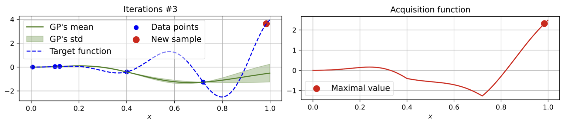
Bayesian optimization applies uncertainty estimation to efficiently search for optimal solutions in complex problem spaces. By maintaining a probabilistic model over possible solutions and iteratively selecting the most uncertain and promising regions to explore, Bayesian optimization has found success in hyperparameter tuning, materials discovery, and drug design. This approach reduces computational costs and accelerates the discovery of optimal configurations.
In reinforcement learning (RL), uncertainty estimation aids in balancing the exploration-exploitation trade-off. In environments where an agent learns through trial and error, uncertainty-aware strategies enable the model to explore unfamiliar states more effectively. For example, in robotics, RL agents guided by uncertainty can discover new control strategies by prioritizing interactions with uncertain states, leading to improved generalization and adaptability.
Across these diverse applications, uncertainty estimation enhances model reliability, efficiency, and robustness. Whether ensuring safety in mission-critical systems or enabling intelligent exploration in decision-making, the ability to quantify and leverage uncertainty is a fundamental aspect of modern deep learning applications.
Conclusion
In this part, we discussed the significance of uncertainty estimation in deep learning and its role in both safety and exploration applications. We explored how uncertainty-aware models enhance decision-making in critical domains such as healthcare, autonomous driving, and financial systems, while also enabling efficient exploration in areas like active learning and reinforcement learning. This is just the beginning—future sections will delve deeper into the technical aspects, methodologies, and advancements in uncertainty estimation, providing a comprehensive understanding of its impact on modern AI systems.
References
[Bis06] C.M. Bishop. “Pattern Recognition and Machine Learning”. Springer, 2006.
[GPM+20] I. J. Goodfellow, J. Pouget-Abadie, M. Mirza, B. Xu, D. Warde-Farley, S. Ozair, A. C. Courville, and Y. Bengio. “Generative adversarial networks”. Communications of the ACM, 2020.
[HG17] D. Hendrycks and K. Gimpel. “A Baseline for Detecting Misclassified and Out-Of-Distribution Examples in Neural Networks”. In International Conference on Learning Representations, 2017.
[HJA20] J. Ho, A. Jain, and P. Abbeel. “Denoising diffusion probabilistic models”. In Advances in Neural Information Processing Systems, 2020.
[HW21] E. Hüllermeier and W. Waegeman. “Aleatoric and epistemic uncertainty in machine learning: An introduction to concepts and methods”, 2021.
[KD09] A. Der Kiureghian and O. Ditlevsen. “Aleatory or epistemic? does it matter?”, Structural safety, 2009.
[KG17] A. Kendall and Y. Gal. “What Uncertainties Do We Need in Bayesian Deep Learning for Computer Vision?”, In Advances in Neural Information Processing Systems, 2017.
[KSM+21] P. W. Koh, S. Sagawa, H. Marklund, S. M. Xie, M. Zhang, A. Balsubramani, W. Hu, M. Yasunaga, R. L. Phillips, I. Gao, et al. “Wilds: A benchmark of in-the-wild distribution shifts”, In International Conference on Machine Learning, 2021.
[LPB17] B. Lakshminarayanan, A. Pritzel, and C. Blundell. “Simple and Scalable Predictive Uncertainty Estimation Using Deep Ensembles”, In Advances in Neural Information Processing Systems, 2017.